INTRODUCTION
The power quality survey is the first, and perhaps most important, step in identifying and solving power problems. Power problems can harm equipment performance and reduce reliability, lower productivity and profitability, and even pose personnel safety hazards if left uncorrected; however, the power quality survey is an organized, systematic way to resolve them. Whether the investigation involves a single piece of equipment or the facility’s entire electrical system, the survey process typically requires these five basic steps:
• Planning and preparing the survey
• Inspecting the site
• Monitoring the power
• Analyzing the monitoring and inspection data
• Applying corrective solutions
• Verify corrective solutions
POWER QUALITY SURVEY TOOLS
The basic tools of the power quality survey are the power quality monitor, circuit tester, multimeter, and an infrared scanner. Other useful tools include clamp-on (Hall effect) current probes, video camera, tape recorder, ground resistance meter, and insulation tester. Not all of these tools are necessary for every survey, but the power quality monitor is the mainstay.
Power quality monitors of widely diverse functionality are available for the documentation of electrical conditions encountered during the physical inspection, as well as the gathering and storing of data for later analysis. Power quality monitors generally fall into two categories: Portable and permanently installed (fixed) systems.
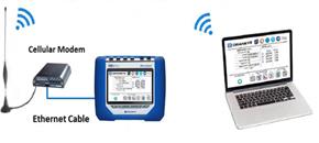
Portable monitors are typically used in temporary applications, and are installed for the duration of the survey and removed upon completion. Such monitors usually have safety (banana jack) connections for voltage and clamp on or Rogowski coil CT’s for current measurements. Survey results can be reviewed on the instrument’s local screen (if available) or uploaded to PC application software, or both. The latest generation of portable monitors enhances user safety and productivity by using Wi-Fi, Ethernet and Bluetooth communications to fully remote control the instrument after the physical installation. Users can close the cabinet door and use their tablet, smartphone, or computer to set up monitoring and review and download data remotely, greatly reducing their exposure to hazardous environments.
Permanent monitors are typically installed for the lifetime of the facility and use screw terminal connections for voltage and split core or solid core CT’s for current measurements. Such monitors are usually safely mounted behind the closed doors of cabinets or switchgear and remotely monitored by server software using an Ethernet or fiber network. Oftentimes, multiple permanent PQ monitors are installed at key points within a facility creating a monitoring system such as at the PCC and at critical loads. Recorded trend and PQ event data is automatically transferred to the server software for use by facility personnel to proactively monitor the quality of supply or to reactively resolve PQ problems as they occur.
Regardless of whether a portable or permanent solution is used, PQ monitors from various manufacturers can have different features and, more importantly, monitoring capabilities and technology. It’s important to make sure that the instrument being used can capture the full spectrum of power quality problems or at least the types of problems suspected. Otherwise, the survey results could be misleading and misreported, wasting valuable time and money.
Modern power quality instruments should be Class A compliant with IEC 61000-4-30 which is an international standard for power quality measurement. Initially released in 2003 and updated in 2008 (next update is pending), IEC 61000-4-30 specifies the measurement techniques that should be employed to appropriately and accurately measure the quality of supply. Being Class A compliant means the instrument fully complies with the standard, is from a reputable manufacturer, and provides accurate and repeatable measurements. Although IEC 61000-4-30 is an international standard, in the United States, the IEEE is in the process of harmonizing to this well-established standard which will be included as part of new editions of IEEE 1159 (power quality) and IEEE 519 (harmonics). An example is the recently released IEEE 519:2014 that adopted the harmonic measurement techniques of IEC 61000-4-7, with added compliance limits for voltage and current.
PLANNING AND PREPARING THE SURVEY
Like any good investigative reporter trying to get to the bottom of the story, the process essentially involves finding out the what, where, when, how, and why of the power related problem(s) at hand. Defining objectives not only keeps the project in focus, but also helps identify the specific equipment resources needed to get the job done. Where to monitor depends on where the problems are observed or suspected. If the problem is localized to one piece of equipment, then placing a monitor at the connection point where the equipment is powered is a good starting point. Sometimes equipment can be both a contributor to and a victim of powering and grounding incompatibilities in the power system. You can then work backward to the point of common coupling (PCC) with the utility if the source of the problem is not found at the equipment. Conversely, if the entire facility is being affected, or if you want to conduct a baseline survey to determine the quality of the supply from the electric utility, starting at the PCC is the logical choice. You can then work down through each feeder circuit to specific loads.
The time when the problem occurs can also provide important clues about the nature of the power problem. If the problem only occurs at a certain time of day, then any equipment switched on at that time should be suspect. Utility operations, such as power factor capacitor switching should also be considered as a potential source of problems that occur regularly and at the same time each day. The monitoring period should last at least as long as a business cycle, which is how long it takes for the process in the facility to repeat itself. Some processes run identically for three shifts, seven days a week. Other operations are different each day of the week, in which case the minimum monitoring period would be one week.
As part of the planning and preparation process, it is necessary to obtain a site history for the facility or equipment being investigated. Asking questions of equipment operators or others familiar with operations is an important part of acquiring the site history. Typical site data of interest would include: determining the time, both occurrence and duration, of recurrent system problems; recording failure symptoms or hardware failures; noting any recent equipment changes, additions, or facility renovations; and logging the operating cycles of major electrical equipment in the facility.
INSPECTING THE SITE
The site examination begins by visually inspecting outside the facility and around the vicinity in order to gain a better perspective of the utility service area. Things to look for include type of electrical service (for example, underground), utility power factor correction capacitor installations, neighboring facilities which might be back-feeding interference onto a shared utility feeder, nearby substations, and other potentially problematic conditions.
Inspecting the facility helps to identify equipment that might cause interference. It will also surface electrical distribution system problems such as broken or corroded conduits, hot or noisy transformers, poorly fitting electrical panel covers, and more. An infrared camera can be very helpful with this. Major electrical loads such as large photocopiers, UPS systems, air compressors, and so forth, should be reviewed. Give special attention to loads near trouble equipment.
Any inspection should include a physical review of the wiring from the critical load to the electrical service entrance to identify any load which might cause power problems. All necessary safety precautions should be observed, such as NFPA 70E, and only qualified personnel should perform any required testing and maintenance work. As Table 1 shows, common wiring problems are a frequent cause of power quality problems. Loose connections and other discrepancies noted during inspection of the electrical distribution system should be corrected prior to monitoring. Particular attention should be paid to equipment power cords and plugs, receptacles, under carpet wiring, electrical panel-boards, electrical conduits, transformers, and the electrical service entrance.
MONITORING THE POWER
The power monitors should be placed at the locations determined during the planning and inspection activities. In general, to determine the overall power quality of the facility, place the monitor at the service entrance. To solve a power problem for a single piece of equipment, place the monitors as close to the equipment load as possible. It’s important to monitor both the voltage and current. Monitoring the voltage identifies the occurrence of a power quality problem, but by also monitoring the current you can determine the source of the problem as either originating upstream or downstream from the equipment load.
The three-step monitoring process involves: (1) using the instrument’s scope mode to see voltage and current magnitudes and wave shapes, (2) using the time interval setting to record background events and slow changes, and (3) using the limits and sensitivity threshold setting to record disturbances or events that may affect the equipment or process being monitored. Periodically checking the captured data allows the user to tweak the thresholds to capture only those events that are critical to the equipment’s performance. (Why capture the entire ocean, when all you want are the fish?)
ANALYZING THE MONITORING AND INSPECTION DATA
To identify equipment problems, it is key to analyze data in a systematic manner. First, look for power events that occurred during intervals of equipment malfunction. Next, identify power events that exceed performance parameters for the affected equipment. Also, review power monitor data to identify unusual or severe events. Finally, correlate problems found during the physical inspection with equipment symptoms. A number of additional procedures must also be performed, including:
• Review all inspection records, site data, and equipment event logs to plot key event summaries.
• Compare power events to equipment event logs and performance specs.
• Extract key power monitoring events which may cause equipment malfunction.
• Classify key power monitoring events into groups to simplify analysis.
• Correlate and validate power monitoring events with equipment symptoms.
• Identify cause in terms of voltage sag, ground or neutral event, transient or voltage distortion (Table 2).
APPLYING CORRECTIVE SOLUTIONS
Adding new wiring, UPS systems, transformers, filters, or other mitigation devices as appropriate may resolve the problems identified during the survey. Moving an interference source to a different circuit sometimes also works. However, make sure that you or the power professional analyzing the survey results has the expertise to safely and properly resolve the problems found. Significant time and money can be wasted deploying inadequate solutions, only to replace them with more appropriate solutions in the future. It is also recommended to repeat the power survey after the problem has been mitigated to prove the problem has been properly resolved and that the power system is now operating as expected.
A more proactive approach is to permanently install a power quality monitoring system at the PCC, each distribution panel, UPS, and each critical load. Monitoring the system in this way produces a more complete, continuous picture of the entire system’s performance. Such systems record power quality (and usually demand and energy) continually and will be online should any problem occur, large or small. Proactive power monitoring can not only be used for continual system improvements and management, but also for automatic notification of a deterioration or change in the power systems, preventing future interruptions, downtime, and lost productivity from occurring.
OBSERVE THE RULES
There are five simple rules to keep in mind while performing a power quality survey:
1. Apply the test of reasonableness to all data and information. Basic laws of physics cannot be temporarily repealed to make something believable.
2. Know the performance as well as the safety limitations of monitoring and test equipment.
3. Look for the obvious. Most power problems are solved like peeling onions – one layer at a time.
4. Don’t fall victim to paralysis by analysis. Set reasonable monitor thresholds, concentrate on the larger events, and then work your way down.
5. Probably the most important rule: start with the simple things first. People are always amazed to find out how often power problems are caused by nothing more mysterious than loose wiring connections. (Table 1).
To find the symptoms, causes, and solutions for the various power events in upper left column, match the adjacent code numbers to the corresponding descriptions in the chart.
Richard P. Bingham retired in 2008 as the VP of Product Development and Marketing for WPT, which includes Dranetz-BMI, Electrotek Concepts, and Daytronic. He presently works as a consultant for Dranetz and PowerCET providing project management, power quality audits, and expert witness. Following completion of his BSEE at the University of Dayton, he joined the company in 1977, and has held positions as project engineer, chief technologist, VP of Engineering, and, VP of Strategic Planning at Dranetz. Richard also has an MSEE in Computer Architecture and Programming from Rutgers University. He is a member of IEEE Power and Energy Society, and the Tau Beta Pi (the Engineering Honor Society). Richard also serves as the chairperson of the IEEE PQ Subcommittee and formerly chair of the NFPA 70B Electrical Equipment Maintenance committee, as well as a principal member of Code Making Panel 20 of NEC on HomeLand Security. He also serves as secretary/vice-chair/chair and member of the numerous other IEEE PQ power quality related committees. He holds one patent.
Ross Ignall graduated from Trenton State College (now The College of New Jersey) in 1986 with a Bachelor of Science in Electronics with a minor in Computer Science. Ross has more than 20 years of experience in the design, development, marketing and application of test and measurement instrumentation. Ross joined Dranetz in 1990 as a Design Engineer, ultimately working as a Group Leader and Senior Engineer leading new product development projects. Ross is presently the Director of Product Management working on the specification, development and application of portable and permanently installed power monitoring instruments and systems.
Ross is a frequent domestic and international speaker and has written many seminars, papers and articles on power instrumentation, power quality, energy monitoring and their applications. Ross is also a contributing author for several books on power quality and power monitoring and is co-inventor of a US patent titled Electrical Parameter Analyzer used as the foundation for Dranetz’ Power Platform family of products.